The Chemist Volume 92 | Number 1
ISSN 1945-0702
Proper Selection and Application of Mathematical Models for Estimating Occupational Exposure to Chemicals Kang Chena,b, Linda F. Martinb aHenkel AG & Co. KGaA, 201203, Shanghai, China. bCapitol Technology University, 20708, Maryland, USA. (* Corresponding author: tjck6@163.com, kchen@captechu.edu)
Abstract: Improper selection and application of chemical exposure models may increase the personnel exposure to hazardous chemicals or lead to a worthless computational effort and unnecessary high-level personal protection. This study is aimed to demonstrate critical points in chemical exposure models selection and application, discuss disadvantages or uncertainties of models with potential opportunities to improve their accuracy, provide equations derivation processes of interest from readers, and introduce advanced chemical exposure modelling software. These objectives are achieved through detailed review and analysis of various models with different level of complexity. It is noteworthy that there is a high potential for predictions to be biased or even become invalid, especially in application of the well-mixed box (WMB) model, near field-far field (NF-FF) model, turbulent diffusion model and Bayesian decision analysis. These critical findings and recommendations can contribute to some reference value for both chemical risk assessment and engineering control in various scenarios of chemical exposure. Key Words: Hazardous chemicals, Chemical exposure, Mathematical modelling, Risk assessment

1. Introduction

Mathematical modelling has been adopted as a primary exposure risk assessment tool given its ubiquitous presence in a range of industries in the past decades. The accelerated pace of the development of computational capability might shed light on the simplification of numerical simulations [1-4]. Today, it could be relatively easy to reach impressive accuracy when establishing simple models thanks to high performance computers.

“All models are wrong, but some are useful” is a famous quote often attributed to the British statistician George E.P. Box. The idea of this quote is that no single model will be perfect or one-size-fits-all, meaning that it will never fully represent the real-world object or process. This leads to the awareness of two limitations of any model, namely the scope of its applicability, and its assumption which is the foundation of incompleteness in information representation. Having said that, even if a model cannot describe exactly the reality it could be fairly useful if it is close enough. Chemical exposure models are of extreme importance to the science and practice of industrial hygiene (IH), and indispensable in implementing exposure risk management programs effectively and efficiently. With robust modelling results, pertinent countermeasures can be proposed for engineering reference to control and reduce hazardous material exposure in various working conditions, even with a very limited exposure sampling number. Furthermore, mathematical modelling can support retrospective exposure estimation for a process that no longer exists, e.g., for the purpose of legal prosecution or epidemiology study. Although models vary in their complexity and application, most of them are time-efficient, cost-effective, and able to diagnose exposures prospectively or retrospectively. Chemical exposure models are also extremely useful as tools for performing quick and preliminary exposure scan that can provide early and timely alert about potential over exposure to hazardous materials in which case further investigations are warranted. On the other hand, if the modelling results suggest that the exposure level is extremely low or trivial, it can also help to prioritize exposure monitoring efforts or justify that there is no necessity for sampling and testing programs. This is critically important considering the high risk and cost of sampling of highly hazardous materials, as well as infeasibility and inaccessibility of industrial hygiene sampling in special working conditions (e.g., in a confined chemical reactor or during transient operations).

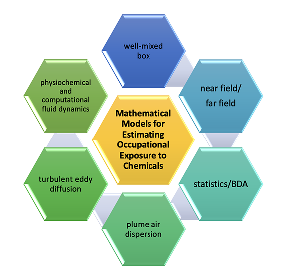
2. Models in Chemical Exposure Modelling Publications

Chemical exposure models, like all other mathematical models, are basically falling into three categories: physics-based, data driven and grey-box models from qualitative, semiquantitative to quantitative [5-7]. While there are numerous modelling text books or tutorial guides in the field of chemical industrial hygiene and occupational health, the publication- “Mathematical Models for Estimating Occupational Exposure to Chemicals (Second Edition)” published by American Industrial Hygiene Association (AIHA) draws great attention from both practitioners and professionals because of its comprehensiveness and practicality. Hereinafter, the name of this publication is abbreviated as “AIHA MMEOEC (Second Edition)”. Its most up-to-date version covers almost all three categories of models, including physics-based models (physiochemical model and computational fluid dynamics model), grey-box models ( well-mixed box model with/without changing conditions, near field/far field two-box model, turbulent eddy diffusion model and plume air dispersion model), and data driven models (statistical model and Bayesian decision analysis). Refer to Figure 1 for demonstration of these models.

Fig 1. Demonstration of Typical Mathematical Models for Estimating Chemical Exposure

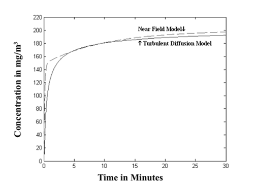
There are multiple opportunities, even for chemical hygiene modelling professionals, to become confused and consequently misunderstand or misapply the principles in model selection and utilization. In this context, the specific purpose of the study is to highlight key points of chemical exposure models selection and application, discuss disadvantages or uncertainties of some models and try to improve their accuracy, identify empirical equations or calculation processes that might lead to misunderstanding or misapplication, demonstrate complete derivation of equations of interest from readers, and introduce newly established modelling and simulation software associated with chemical exposure. In the following sections, all these topics will be discussed respectively in details. While this study was performed mainly based on the AIHA mathematical modelling book, a wider range of topics are analyzed and discussed further in details, and the conclusions could be valuable for both risk assessment and engineering control of hazardous material exposure.

3. Key Points in Chemical Exposure Models Selection and Application

3.1 For a relatively complex indoor environment, the total volume of rooms might be divided into smaller volumes or determined by displacing all solid objects in the room. In many cases of a real chemical laboratory environment, the displaced volume could be significant, but this is often neglected or simplified incorrectly by chemists, which can lead to underestimation of actual concentrations of airborne pollutants and consequently overexposure to hazardous materials due to inadequate protective actions being taken based on the modelling results. It is imperative to raise awareness for all chemists to acquire real data on room volume when the well-mixed room model or computational fluid dynamics model is utilized. Furthermore, in these models, the concentration of contaminants in the make-up air is usually assumed to zero. This might not be true when the outdoor ambient environment is highly polluted together with high potential of outdoor airflow infiltration or reentry into the built environment.

3.2 The well-mixed model is widely recognized as the easiest approach to modeling the indoor chemical contaminant concentrations. Nevertheless, it is a useful approach only if the room air is, indeed, well-mixed or if the contaminant is released at multiple locations throughout a room [8]. The use of mixing factors is discouraged from the author’s perspective because they defy the law of conservation of mass and cannot be adequately quantitative. For example, the impact from airflow short circuits might not be mitigated by using a mixing factor and thus variations in pollutant concentration are still exist in the room.

3.3 Although air change is not addressed in the turbulent eddy diffusion models, such kind of removal mechanism in the vicinity of the emission source (e.g., within 1 meter), could be negligible in reducing exposure intensity [9]. Thus, in general, turbulent diffusion models are used to evaluate exposure profile in the near field with the following rules of thumb:

• The concentration value becomes infinite when the distance from the source approaches zero, but an infinite concentration is impossible in the real situation. Thus, the turbulent diffusion models are not appropriate for positions very close to the emission source (e.g., less than 10 cm) [9].
• The turbulent diffusion coefficient (DT) needs to be calculated carefully and accurately in order to obtain consistent results with the near field (NF) model.
• Contaminants should be released freely without high pressure and thermal energy. Specifically, modeling dispersion via advective air flow and turbulent diffusion is much more difficult than if there is no advective flow due to lack of a closed-form equation that describes the contaminant concentration at various locations and time periods [10-11]. This might answer the question that why only the steady state (time-independent) concentrations are calculated in the current IHMOD software [12].
• Cross-drafts and middle-field effects are not considered in the near field and far field (NF-FF) model, which leads to less adaptability in terms of the concentration gradients compared with the turbulent diffusion model. Figure 2 [9] demonstrates the difference in pollutant concentration gradients within the first 5 mins for a real case of toluene exposure. The NF-FF model is mainly applied to scenarios of exposure to chemicals with acute toxicity, especially in an imperfectly mixed indoor environment.

Fig 2. The Comparison of Concentrations as Predicted by the Near Field/Far Field Model Versus the Hemispherical Turbulent Diffusion Model for a Toluene Emission Scenario

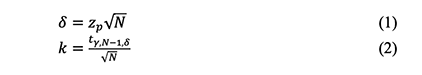
3.4 A recently developed modelling freeware (Expostats) for Bayesian decision analysis (BDA) has drawn great attention from the chemical hygiene community [13-15]. BDA has been used in the interpretation of chemical exposure measurements as it renders quantitative integration of professional judgement [16-19] together with data gained from numerical simulations or previous measurements, which permits us to calculate decision probabilities with small sample sizes, even for a single measurement [20-21]. As it is claimed that comparing arithmetic mean to the chemical occupational exposure limit (OEL) is less conservative than comparing the exceedance fraction to 5%, this new tool selects the latter criteria which is numerically equivalent to comparing the estimated 95th percentile to the OEL. Compared with several tools mentioned in the AIHA MMEOEC (Second Edition) (e.g., IHSTAT and IH Data analyst), its assessment output is presented through a risk gauge with a needle indicating the probability value within the related risk category, which can facilitate an easy understanding of the pertinent exposure risk even for general public. Another merit is that this toolkit extends from only left-censored data to interval- and right-censored data and can complete the pretreatment of non-detects in chemical hygiene samples [22-24]. Suitability of the lognormal model for the case under investigation is one important limitation of this tool, and readers might need to consider quasi nonparametric upper tolerance limits (UTLs) for exposure evaluations if measurement results are predominantly below the exposure limit or if their distribution cannot be assumed to comply with parametric assumptions [25].

4. Disadvantages or Uncertainties of Models and Solutions to Improve Their Accuracy

4.1 In the example 2.4 in the AIHA MMEOEC (Second Edition), the total volume of compressed gas released to the indoor environment is simply calculated by nominal cylinder volume times the ratio between gas cylinder internal pressure and external atmospheric pressure. Nevertheless, chemical industrial standards suggest that the coefficient of compression for the gas investigated under different temperature and pressure should be considered during the calculation to address the real situation [26], through which the final leakage concentration could be obtained more accurately.

4.2 Although the equation (6-3) and (6-4) in the AIHA MMEOEC (Second Edition) describe the time-dependent chemical concentrations in the near and far field, respectively, it is recommended to consider the variability of contaminant generation rate, especially when temperature plays an important role (e.g., large-scale outdoor coating operation during different time periods in a day). In such kind cases, the relationship between temperature and time, i.e., temperature ~ F(time), should be setup firstly and then refer to the equation 6 in this study to establish the function expression between the contaminant generation rate (G) and time, i.e., G ~ f (temperature) ~ f (F(time)).

4.3 The AIHA IHSTAT software uses the Natrella formulas to derive the tolerance factor k in calculating UTL 95%, 95%, in which case the chemical samples number should be relatively large (e.g., more than 10) in order to keep adequate accuracy of the modelling outputs [27,28]. It is recommended that pertinent alert should be posted regarding the requirement of the sampling size in the user guide, or preferably another algorithm based on non-central t-distribution might be utilized to obtain more accurate results for smaller sampling quantity [28,29]. The major improvement of this alternative algorithm lies in its calculation of the approximate tolerance factor k for one-sided tolerance intervals by the following set of formulas:

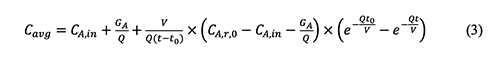
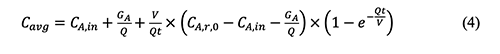
where δ is the non-centrality parameter, Z_p is the critical value of the normal distribution, γ is the probability and N is the number of sampling.

5. Derivation Process of Empirical Equations in Chemical Exposure Modelling

5.1 The general form of the equation (4-20) in the AIHA MMEOEC (Second Edition) for determining the average exposure concentrations over time is shown below based on the author’s derivation process as well as another teaching note from Mark Nicas [30].

Where:

C_avg: Time-averaged concentration of chemical A in room air
C_A,in: Concentration of chemical A in supply air
G_A: Generation rate of chemical A
Q: Ventilation rate
t: Time, t₀: Initial time
C_A,r,0: Concentration of chemical A in room air at time t₀

By integrating the well-mixed box (WMB) equation above from time t = 0 to time t = t, it could be easy for readers to find that the equation (4-20) in the AIHA MMEOEC (Second Edition) is incorrect and its right form can be derived as below:

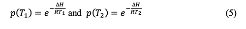
Further, the limitation of the current equation (4-20) in the AIHA MMEOEC (Second Edition) is that it can only be applied for the scenario t₀ = 0. Without reminders or application notes, readers may assume that this equation can be applied to all scenarios just because t₀ and t can be defined as any value, and consequently incorrect average exposure concentrations are obtained.

5.2 The derivation process of the equation for calculating emission rate under various temperature in the example 5.1 and the equation (5-14) in the AIHA MMEOEC (Second Edition) are shown below, respectively, in detail.
Transform the Clausius-Clapeyron equation [31,32] ;
then change the differential part into its derivative form, we obtain  ,
 , using T1 and T2 representing two different temperatures, the following equations are derived:

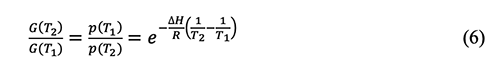
Where:

∆H is the molar enthalpy of vaporization, R is the molar gas constant, p(T₁), and p(T₂) are the vapor pressure under the absolute temperature T₁ and T₂, respectively.

Finally, the relationship between the emission rate G(T) and the room temperature is expressed as:

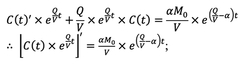
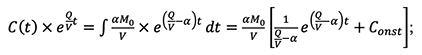
5.3 The derivation process of the equation (5-14) in the AIHA MMEOEC (Second Edition) hereinafter is relatively complex:

Step one, rewrite the equation (5-13) in the AIHA MMEOEC (Second Edition) as: ;

Step two, insert the exponential term in order to formalize the derivative term below:

Step three, by integrating both left and right side of the equation above, the following transformation can be derived:

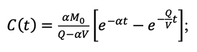
Step four, based on previous assumption C(0) = 0 and thus the constant of integration C_onst can be obtained as 1/(α-Q/V);

Finally, rearrange all the terms and the equation (5-14) is obtained as

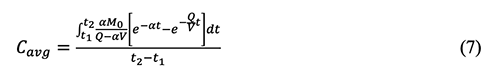
Further, the integral form of the equation (5-14) should be constructed in order to know the time averaged concentration without consideration of back-pressure as below.

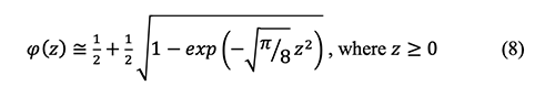
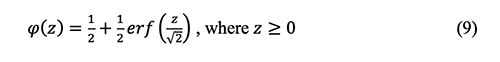
Where  is the emission rate constant, M₀ is the initial contaminant mass in the source, all the other parameters are the same as those defined in the equation 3, previously.

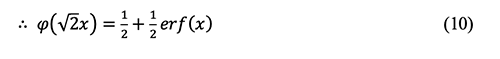
and the relationship between the error function and  is:

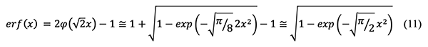
To eliminate , let  , then  

The above equations 8 and 10 are coupled in order to solve the error function as below:

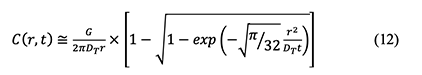
Finally, the following concentration equation in terms of radial distance r from the pollutant emission source and time t is derived and provides values close to those computed by the exact equation based on the error function:

While there are no details on derivation of the equation (7-9) in the AIHA MMEOEC (Second Edition), the equation 12 above provides relatively accurate and easy understanding reference on solving the chemical turbulent eddy diffusion model.

6. Misleading or Incomplete Information

6.1 The US EPA website linkage provided in the section 3.4 “Evaporation from Open Surfaces” of the book is not valid and the correct on-line resource for the molecular diffusion coefficient in the air should be directed to: https://www3.epa.gov/ceampubl/learn2model/part-two/onsite/properties.html, and then select “Diffusivity in air and water” column for more details.

6.2 The parameter “K₁XV” in Rule #19a in the Appendix I and the factor K in the equation (4-8) in the AIHA MMEOEC (Second Edition) should be consolidated as “K_sink” as both of them have the same meaning to represent the rate of contaminant loss through sinks [36-38], through which can enhance content coherency and readership.

7. Discussion and Conclusion

In this article, multiple mathematical models for chemical occupational exposure evaluation are reviewed systematically and analyzed further in terms of model election, output accuracy and derivation process, which facilitate a better understanding and correct application of different models for chemists or chemical engineers. There are numerous tricks and traps for chemical practitioners or professionals to make imperfect or even incorrect decisions, especially using the WMB model, turbulent eddy diffusion model, NF-FF model, statistical model and Bayesian decision analysis as explained and highlighted above. This critical analysis shines new light onto the application and optimization of mathematical models for chemical occupational exposure evaluation through demonstrating how model predictions could be biased and effective solutions to prevent those misapplications.

There are some recognized challenges or limitations in the present research, which should be addressed in future work. Chemical exposure models investigated in this study only represent a relatively small number of models in real applications due to either research focus or resource limitation. There may be a wider range of exposure scenarios in the emerging chemical industries, including but not limited to exposure to nanoparticles, radioactive chemicals, active pharmaceutical ingredients (APIs) and biochemical active substances (BAS). Recommendations for future work include, first, research on mathematical modelling of dermal exposure to chemicals should be encouraged and scrutinized because physical exposure measurement can be quite challenging considering the uncertainties associated with attempting to quantify real dermal exposure. Currently, there is no scientific method or “golden standard” of measuring the results of the body’s exposure to chemicals through dermal contact [39,40]. Therefore, it provides great opportunity and space for the application of dermal exposure models to the chemical community. Additionally, the emerging topic on modelling of combined physiochemical exposure becomes promising and deserve to be further analyzed (e.g., ototoxic chemicals and noise) [41-43].  Last but not least, it is equally important to develop a good mathematical model than knowing how to interpret the results. And here is where the expert interactions are more needed, knowing how to illustrate the results successfully to not only the chemical practitioners but also the general workforce who are concerned with their personal exposure to chemicals.

Acknowledgments

The authors thank Prof. Jérôme Lavoué from University of Montreal, Christopher Packham, FRSPH, FIIRSM from EnviroDerm Services and Dr. Paul Hewett from Exposure Assessment Solutions, Inc. for their technical guidance and professional comments in the field of chemical exposure modelling.

1. Shiling Z, Paul P, Liangbo H, Parmesh V, Richard L, Larry B. “CFD modeling of flammable refrigerant leaks inside machine rooms: Emergency ventilation rates for different size chillers". Sci. Technol. Built Environ., 2018, 24(8), 878-885. DOI: 10.1080/23744731.2018.1448676.
2. Stern F, Wilson RV, Coleman HW, Paterson EG. “Comprehensive approach to verification and validation of CFD simulations—part 1: methodology and procedures”. J. Fluids Eng., 2001, 123(4), 793-802. DOI: 10.1115/1.1412235.
3. Chen K, Yang JL, Zhang HB, Zhang WJ. “Low level noise analysis in laboratory fume hood”. J. Chem. Health Saf., 2017, 24(1), 2–7. DOI: 10.1016/j.jchas.2016.03.002.
4. Kang C, Weize W, Wenjun Z. “Investigation of influential factors on laboratory fume hood containment performance”. Sci. Technol. Built Environ., 2020, 26(3), 387-399. DOI: 10.1080/23744731.2019.1637192.
5. Abdul A, Farrokh JS. “Review of modeling methods for HVAC systems”. Appl. Therm. Eng., 2014, 67(1–2), 507-519. DOI: 10.1016/j.applthermaleng.2014.03.055.
6. Abdul A, Farrokh JS. “Gray-box modeling and validation of residential HVAC system for control system design”. Appl. Energy, 2015, 137, 134-150. DOI: 10.1016/j.apenergy.2014.10.026.
7. Abdul A, Farrokh JS. “Black-box modeling of residential HVAC system and comparison of gray-box and black-box modeling methods”. Energy Build., 2015, 94, 121-149. DOI: 10.1016/j.enbuild.2015.02.045.
8. Heinsohn RJ in “General Ventilation Well-Mixed Mode”, Industrial Ventilation Engineering Principles, John Wiley & Sons, Inc., New York, 1991, ch. 5. ISBN-13: 978-0471637035.
9. American Industrial Hygiene Association in Mathematical Models for Estimating Occupational Exposure to Chemicals, American Industrial Hygiene Association, Virginia, 2009. ISBN: 978-1-935082-10-1.
10. Nicas M, Armstrong TW. “Computer implementation of mathematical exposure modeling”. Appl. Occup. Environ. Hyg., 2003, 18(8), 566–571. DOI: 10.1080/10473220301417.
11. Nicas M. “Modeling turbulent diffusion and advection of indoor air contaminants by Markov chains”. Am. Ind. Hyg. Assoc. J., 2001, 62(2), 149-158. DOI: 10.1080/15298660108984617.
12. http://www.aiha.org/Content/InsideAIHA/Volunteer+Groups/EAScomm.htm, AIHA IH MOD software, accessed 9/8/2020.
13. Jérôme L, Lawrence J, Peter K, Hugh D, France L, Frédéric C, Gautier M, Tracy K. “Expostats: A Bayesian toolkit to aid the interpretation of occupational exposure measurements”. Ann. Work Exposures Health, 2019, 63(3), 267–279. DOI: 10.1093/annweh/wxy100.
14. Gurumurthy R. “Progress in Bayesian statistical applications in exposure assessment”. Ann. Work Exposures Health, 2019, 63(3), 259–262. DOI: 10.1093/annweh/wxz007.
15. Eun GL, Diana MC. “Adoption of exposure assessment tools to assist in providing respiratory protection recommendations”. Ann. Work Exposures Health, 2020, 64(5), 547-557. DOI: 10.1093/annweh/wxaa023.
16. Susana GH, Mariscala MA, Javier GR, Dale OR. “Working conditions, psychological/physical symptoms and occupational accidents. Bayesian network models”. Saf. Sci., 2012, 50(9), 1760-1774. DOI: 10.1016/j.ssci.2012.04.005.
17. Ramachandran G, Vincent JH. “A Bayesian approach to retrospective exposure assessment”. Appl. Occup. Environ. Hyg., 1999, 14(8), 547–557. DOI: 10.1080/104732299302549.
18. Sottas PE, Lavoué J, Bruzzi R, David V, Nicole C, Droz PO. “An empirical hierarchical Bayesian unification of occupational exposure assessment methods”. Stat. Med., 2009, 28(1), 75–93. DOI: 10.1002/sim.3411.
19. Banerjee S, Ramachandran G, Vadali M, Sahmel J. “Bayesian hierarchical framework for occupational hygiene decision making”. Ann. Occup. Hyg., 2014, 58(9), 1079–1093. DOI: 10.1093/annhyg/meu060.
20. Jones RM, Burstyn I. “Bayesian analysis of occupational exposure data with conjugate priors”. Ann. Work Exposures Health, 2017, 61(5), 504–514. DOI: 10.1093/annweh/wxx032.
21. Paul H, Perry L, John M, Gurumurthy R, Sudipto B. “Rating exposure control using Bayesian decision analysis”. J. Occup. Environ. Hyg., 2006, 3(10), 568-581. DOI: 10.1080/15459620600914641.
22. https://expostats.ca/site/app-local/NDExpo, NDExpo, a JavaScript Web application that implements the robust ROS (regression on order statistics) censored data treatment approach, accessed 9/8/2020.
23. Dennis RH in “Computing Summary Statistics and Totals”, Statistics for Censored Environmental Data Using Minitab® and R, 2nd Edition, Wiley, New Jersey, 2012, ch. 6. ISBN: 978-0-470-47988-9.
24. Dennis RH. “More than obvious: better methods for interpreting nondetect data”. Environ. Sci. Technol., 2005, 39(20), 419A–423A. DOI: 10.1021/es053368a.
25. Charles BD, Paul FW. “‘Quasi Nonparametric’ upper tolerance limits for occupational exposure evaluations”. J. Occup. Environ. Hyg., 2015, 12(5), 342-349. DOI: 10.1080/15459624.2014.995301.
26. CSBTS (China State Bureau of Quality and Technical Supervision). Industrial nitrogen (GB/T 3864-2008). CSBTS: Beijing, China, 2008.
27. Selvin S, Rappaport SM, Spear R, Schulman J, Francis M. “A note on the assessment of exposure using one-sided tolerance limits”. Am. Ind. Hyg. Assoc. J., 1987, 48(2), 89-93. DOI: 10.1080/15298668791384445.
28. National Institute of Standards and Technology (NIST). Product and Process Comparisons, NIST/SEMATECH e-Handbook of Statistical Methods, NIST, Maryland, 2013, ch. 7. DOI: 10.18434/M32189.
29. CSBTS (China State Bureau of Quality and Technical Supervision). The tables of quantiles of the noncentral t-distribution (GB/T 15932-1995). CSBTS: Beijing, China, 1995.
30. Nicas M. PH 270A Indoor Air Quality Models, teaching notes, 2020.
31. David RL in CRC Handbook of Chemistry and Physics (82nd Edition), CRC Press, Inc., Florida, 2001. ISBN: 978-0849304828.
32. John AD in Lange′s Handbook of Chemistry (15th Edition), McGraw-Hill, Inc., New York, 1999. ISBN: 0-07-016384-7.
33. Aludaat KM. “Alodat M.T. A note on approximating the normal distribution function”. Appl. Math. Sci., 2008, 2(9), 425-429.
34. Eidous OM, Shareefa RA. “New approximations for standard normal distribution function”. Commun. Stat.—Theory Methods, 2020, 49(6), 1357-1374. DOI: 10.1080/03610926.2018.1563166.
35. Wang JJ, Yang ZL. “Review of approximating functions to cumulative normal distribution function”. J. Comput. Appl. Math., 2014, 34(S2), 83-84, 90. DOI: 1001-9081(2014)S2-0083-02.
36. Jayjock MA, Doshi DR, Nungesser EH, Shade WD. “Development and evaluation of a source/sink model of indoor air concentrations from isothiazolone-treated wood used indoors”. Am. Ind. Hyg. Assoc. J., 1995, 56(6), 546-557. DOI: 10.1080/15428119591016773.
37. Salma I, Dosztály K, Borsós T, Söveges B, Weidinger T, Kristóf G, Péter N, Kertész Zs. “Physical properties, chemical composition, sources, spatial distribution and sinks of indoor aerosol particles in a university lecture hall”. Atmos. Environ., 2013, 64, 219-228. DOI: 10.1016/j.atmosenv.2012.09.070.
38. He C, Morawska L, Gilbert D. “Particle deposition rates in residential houses”. Atmos. Environ, 2005, 39(21), 3891-3899. DOI: 10.1016/j.atmosenv.2005.03.016.
39. European Agency for Safety and Health at Work (EU-OSHA). Occupational skin diseases and dermal exposure in the European Union (EU-25): policy and practice overview, EU-OSHA, Belgium, 2008. ISBN: 978-92-9191-161-5.
40. Konstantinos MK, Suzanne S, Angelos NT, Remy F, Ilianna C, Pelagia A, Kyriaki M, Dag R, Michael R, Ulrich P, Gianna L, Anja B, Urs S, Rianda MGE. “Comparison of measurement methods for dermal exposure to hazardous chemicals at the workplace: the SysDEA project”. Ann. Work Exposures Health, 2020, 64(1), 55–70. DOI: 10.1093/annweh/wxz085.
41. Chen K, Zhang HB, Zhang WJ. “Measures to alleviate fume hood noise”. Am. Lab., 2018, 50(3), 10-13.
42. Chang SJ, Chen CJ, Lien CH, Sung FC. “Hearing loss in workers exposed to toluene and noise”. Environ. Health Perspect., 2006, 114(8), 1283–1286. DOI: 10.1289/ehp.8959.
43. Choi YH, Kim K. “Noise-Induced hearing loss in Korean workers: Co-Exposure to organic solvents and heavy metals in nationwide industries”. Plos One, 2014, 9(5), e97538. DOI: 10.1371/journal.pone.0097538.