|
Introduction The development of hollow-fibre membranes during the 1970s helped reverse osmosis (RO) technology advance even further. Since the early development of RO membranes for sea water desalination, hollow-fibre membranes have been crucial to membrane separation technology. This is mainly because of their large surface area, which typically exceeds other membrane module configurations (104 m2/m3 per unit volume). They are also independent (there is no need for supporting material). To be able to endure high operating pressure for RO applications without collapsing, hollow-fibre membranes for RO desalination are typically of tiny fibre size in the range of 50 - 300 μm outer diameter [1]. The fibers are typically referred to as hollow-fine-fibers when their diameter falls between 50 and 500 μm. They can tolerate intense feed pressure (20 bar or higher) applied from the outside [2]. They are suitable for RO or high-pressure gas separation due to this characteristic. Hollow-fibers are frequently utilized for microfiltration (MF) or ultrafiltration (UF), which do not require significant operating pressure [3]. For the preparation of hollow-fiber membranes, the dry-wet spinning method is frequently used. This spinning process can be employed to obtain almost every known membrane morphology by controlling the phase separation processes that take place. According to Tawari and Brika, 2018, three spinning parameters including solvent/non-solvent ratio, bore fluid composition and air gap distane may have an effect on the fibre morphology [1]. In order to investigate the effects of the spinning parameters (factors) on the fabrication process, factorial design was performed. Factorial design and the associated analysis of variance are useful tools to characterize processes which are influenced by a number of factors. The methods allow the determination of statistically important factors and enable the experimenter to study the joint effect of the factors on the response [4]. In this way, a regression model for each of the measured can be generated. In this study, a 33–factorial design [3] is used to identify which factors and their interactions have the most important effect of the performance of CA hollow-fine-fibre membrane for brackish water desalination.
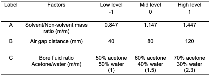
Experimental Design Based on literature and preliminary results obtained in previous work of the authors [1], three important factors which affect the fabrication process were considered: solvent/non-solvent ratio, air gap distance and bore fluid composition. Each factor will be studied at three levels, and a 33 full factorial design was selected to achieve this goal because it consists of all possible combinations of the levels for all factors. It is also useful for investigating quadratic effects, which is not possible with 2 level design. The responses of interest are (flux) and (retention). The list of factors and their chosen levels for the experiment are shown in Table 1. The hollow-fine-fibre membrane performance was determined using an applied pressure of 20 bar and a feed solution of 2,000 ppm (NaCl).
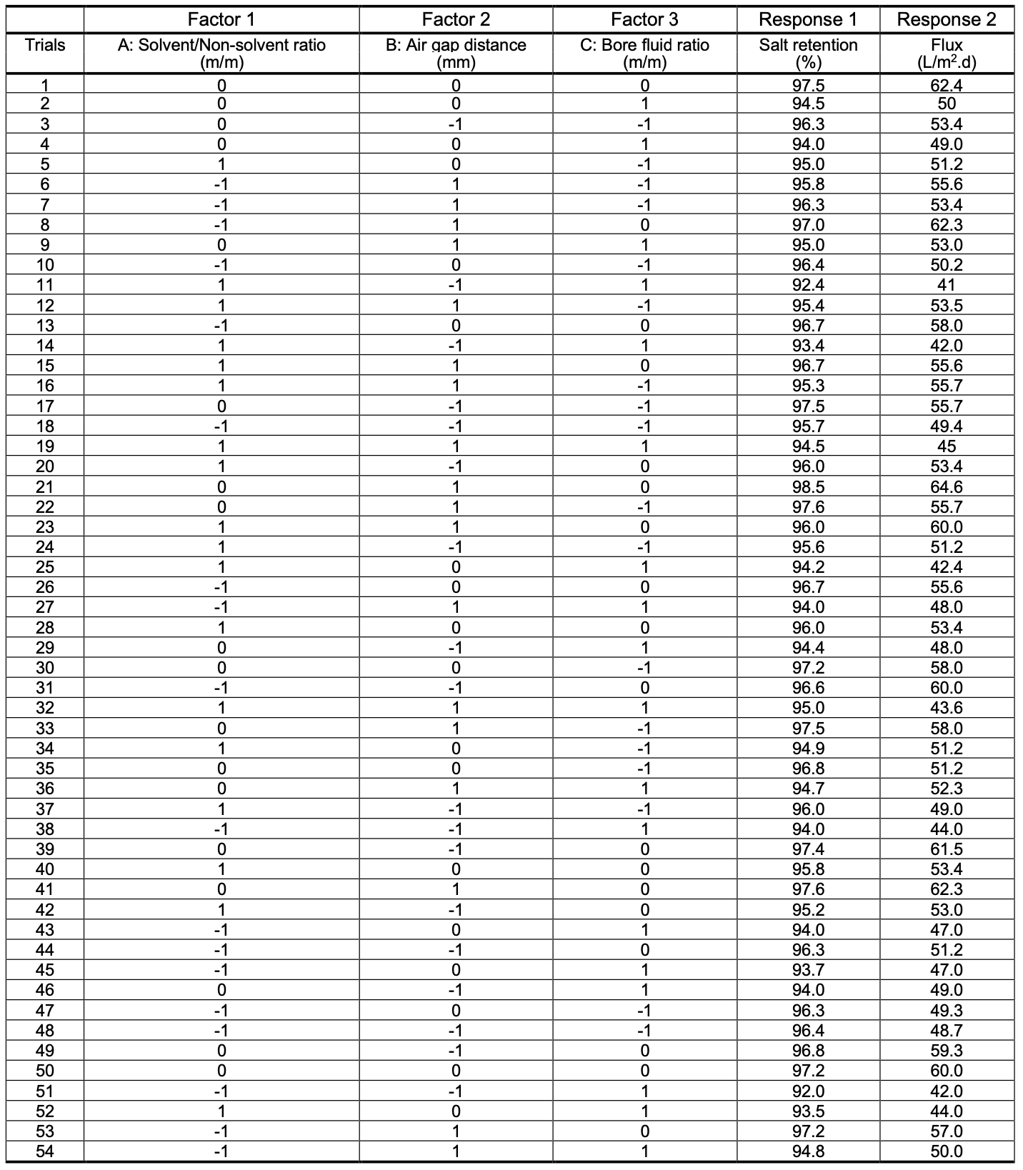
Each trial was replicated twice since replication permits more degrees of freedom in the estimation of error variance and provides the means to determine variability between treatments and that due to random variation. The Design-Expert Software 7.1 was used to analyze the experimental data. The experimental results of the 33–factorial design are shown in standard order in Table 2.
Results and Discussion The salt retention and permeate flux responses for each experimental trial are shown in Table 2. These results were statistically analyzed using analysis of variance (ANOVA) to study the joint effect of each factor and their interactions on the membrane performance (retention and flux). Analysis of Variance (ANOVA) This method was first developed by Fisher in 1930 [5]. ANOVA is a statistical method used to evaluate which of the factors studied significantly affects the responses over the range studied [6]. The relative importance of each factor and factor-factor interaction can be ranked in terms of their effect on the process output. Thus, the information about how significant the effect of each factor on the experimental results can be concluded from ANOVA. Tables 3 and 4 summarize the ANOVA of the three factors studied.
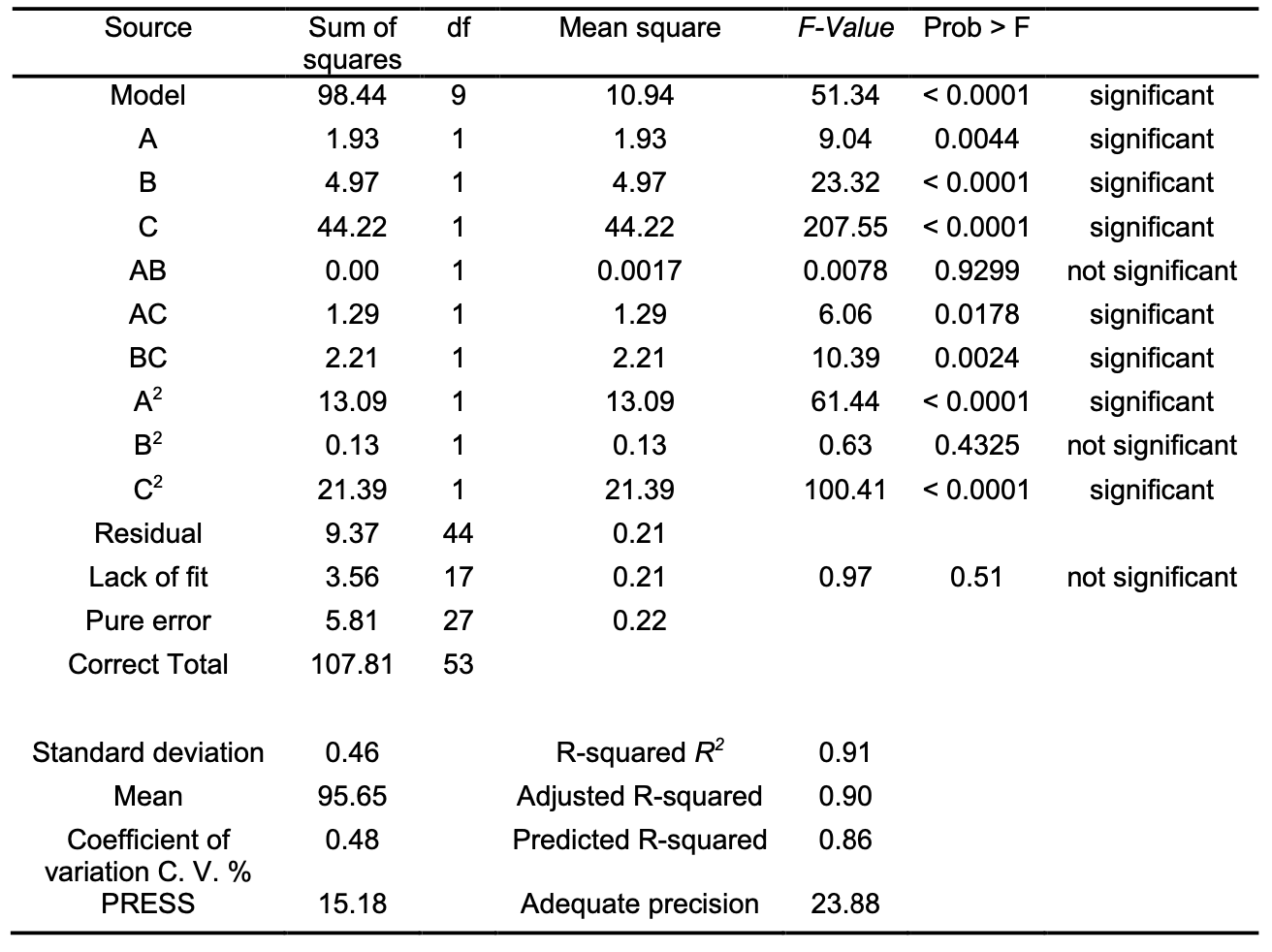
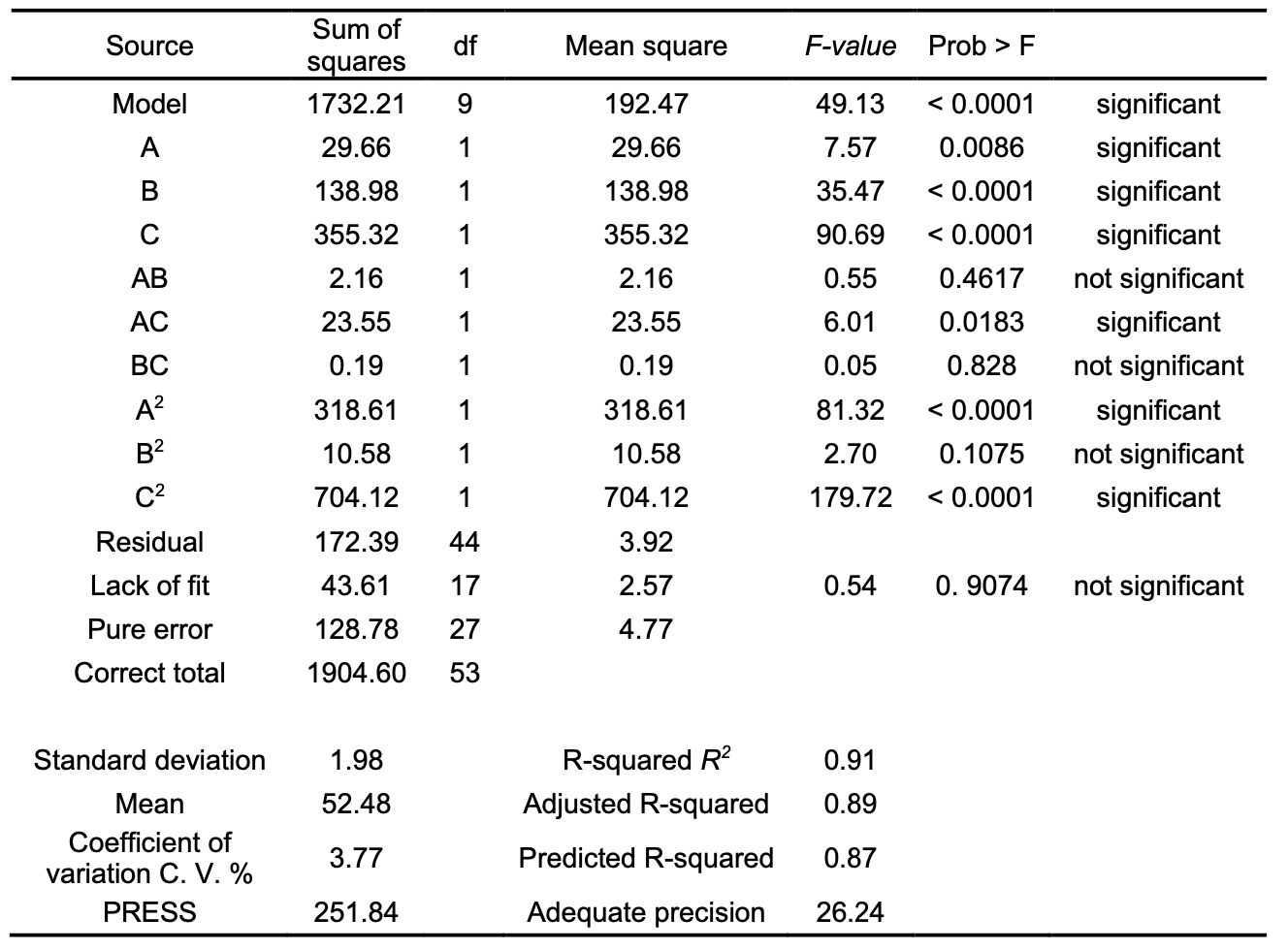
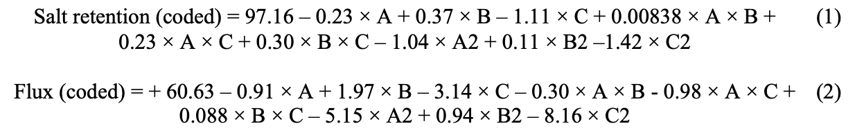
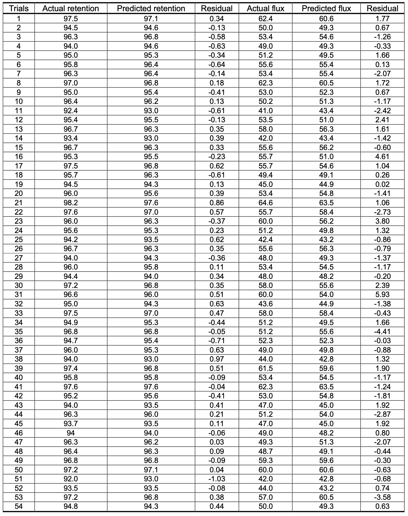
Checking the Adequacy of Both Regression Models In Tables 3, 4, the “Model F-values” are calculated from a model mean square divided by residual mean square; the residuals are defined as the differences between the experimental data and the predicted values for each point in the design. The Model F-value is the test for comparing model variance with residual (error) variance. If the variances are close to the same, the ratio will be close to one and it is less likely that any of the factors have a significant effect on the response. Similarly, an “F-value” for any individual factor terms is calculated from a term mean square divided by a residual mean square. It is a test that compares a term variance with a residual variance. If the variances are close to the same, the ratio will be close to one and it is less likely that the term has a significant effect on the response. In Table 3, a “Model F-values” of 51.34 with a “Model F-values” 49.13 in Table 4 imply that the selected models are significant and there is only a 0.01% chance that a “Model F-values” this large could occur due to noise. Prob > F represents the probability of seeing the observed F value if the null hypothesis is true (there is no factor effect). Small probability values call for a rejection of the null hypothesis. The probability equals the proportion of the area under the curve of the F-distribution (with 9 and 27 degree of freedom) that lies beyond the observed F-value. Furthermore, the P-value is the probability that the test statistic will take on a value that is at least as extreme as the observed value of the statistic when the null hypothesis is true. Thus, a P-value conveys much information about the weight of evi- dence against null hypothesis, and so a deci- sion maker can draw a conclusion at any specified level of significance. More formally, we define the P-value as the smallest level of significance that would lead to the rejection of the null hypothesis [7,8]. In other words, if the Prob > F value is very small (less than 0.05), then the terms in the model have a significant effect on the response, providing at least 95% confidence for results. If the Prob > F value is greater than 0.1 then this is an indication that the model terms are not significant. The “lack-of- fit F-values” for both models implies that the lack of fit is not significantly related to pure error. These values of lack of fit are desirable as we want to know how well the models fit the experimental data. “R-squared”, or more formally the coefficient of multiple determination, is defined as the sum of squares for the model divided by the total corrected sum of squares and indicates the proportion of the variability in the data explained by the analysis of variance model [9]. The R2 values of models were calculated to be 0.91 in both instances, indicating that only 9% of the total variation was not explained. Thus, the models were able to explain about 91% of the variability in salt retention and permeate flux data. The closer the value of R2 is to unity, the better is the correlation between the observed and predicted values [10]. In this study, the predicted R2 of 0.86 and 0.87 are in reasonable agreement with the adjusted R-squared of 0.90 and 0.89 of both models. Adequate precision measures the signal to noise ratio. A ratio greater than 4 is desirable. Adequate precisions of 23.88 and 26.24 for both models indicate adequate model discrimination [4]. The coefficient of variation (CV) for the re- tention and flux were calculated to be 0.48 and 3.77%. The CV, the ratio of the standard error of estimate to the mean value of the observed response (as a percentage), is a measure of reproducibility of the model and, as a general rule, a model can be considered reasonably reproducible if its CV is not greater than 10% [11,12]. The predicted sum of squares (PRESS), which is a measure of how a particular model fits each point in the design, was 15.18 and 251.84. According to Table 3, the main factors of A, B, C, the interaction of AC, BC, and the second orders of A2, C2 are significant model terms. In Table 4, the main factors of A, B, C, the interaction of AC and the second orders of A2, C2 are significant model terms. The other factors are less significant but cannot be neglected due to their little influence on responses as well. The results of each of these overall responses are included in the analysis procedure and an equation that describes the influence of the factors on the overall responses was found. The following equations are the final regres- sion models in terms of the actual and coded factors. Table 5 tabulates the differences be- tween the actual and predicted response values according to the equations.
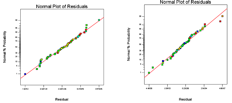
In order to check data for normality, even when there is fairly small number of observations, it is best to construct normal probability plots of the residuals. Here “residual” means the difference in the observed values (obtained from the experiments) and the predicted value or fitted values. The normal probability plot shows the residuals plotted against a cumulative normal percentile derived from the normal probability distribution for the ranking location of the residuals. This provides a visual method to illustrate if the residuals are actually normally distributed. If the residuals fall approximately along a straight line, the residuals are then normally distributed. In contrast, if the residuals do not fall fairly close to a straight line, the residuals are then not normally distributed and hence the data do not come from a normal population. In Table 5, the residuals are ranked in ascending order from the lowest to highest in order to plot the normal probability plot and their cumulative probability points are calculated Pk= (K – 0.5)/n, where K is the sequence number from 1 to n and n is the number of entries in the list.
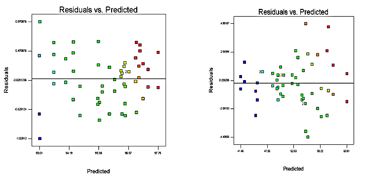
Figure 1 shows the normal probability plots of the residuals. There is no indication of nonnormality, nor is there any evidence pointing to possible outliers. It can be concluded that the normal distribution provides an excellent model for the data. The next residual plot which we examine was the plot of residuals versus the predicted values in Figure 2. The plot of the residuals versus the ascending predicted response values indicated that there is no expanding variance phenomenon.
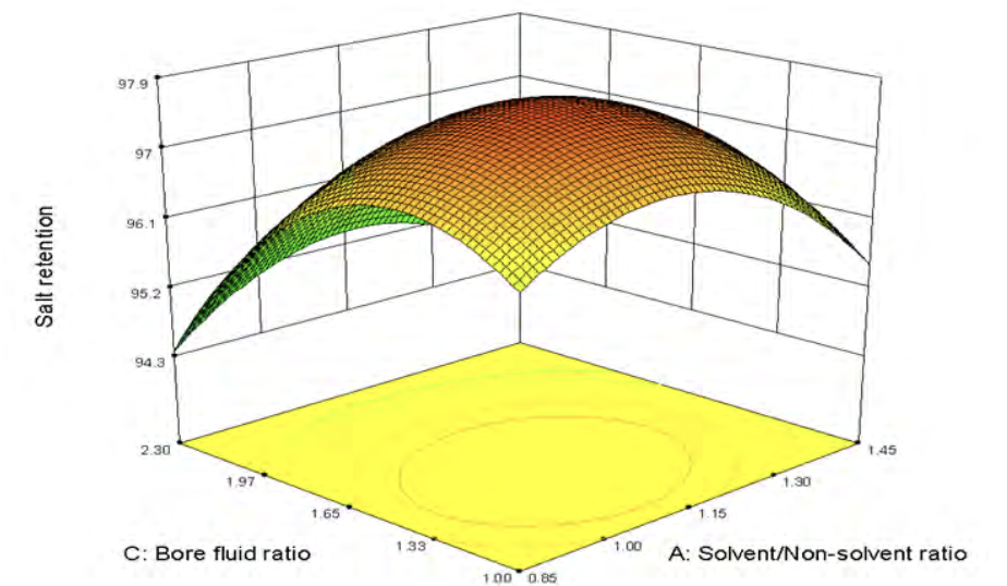
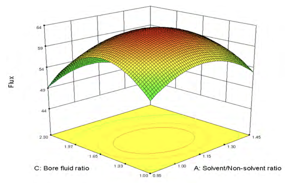
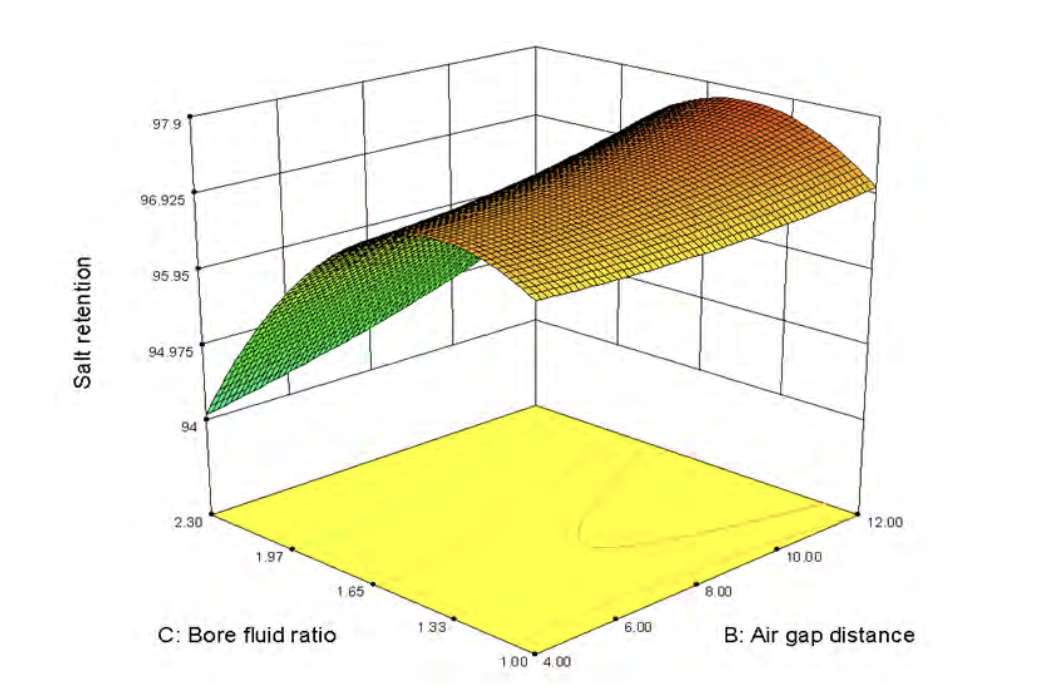
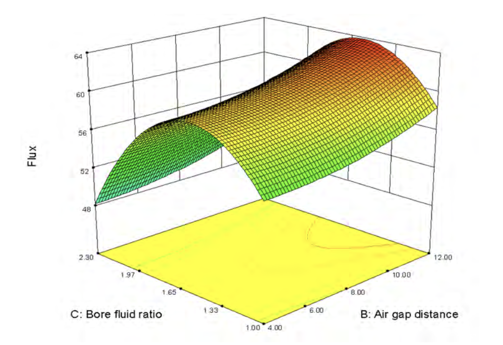
The residual values seem to be randomly scattered above and below zero over the range of the data and do not indicate any problems with the model. The reference line at 0 emphasizes that the residuals are split about 50-50 between positive and negative. There are no systematic patterns or unusual structures apparent in this plot. Plots in which the residuals do not exhibit any systematic structure indicate that the model fits the data well. In contrast, plots of the residuals that exhibit systematic structure indicate that the form of the function can be improved in some way [1]. Therefore, Figure 2 indicates that the model fits and there is no reason to suspect any violation of the independence or constant variance assumption. Effect of Factors and Interactions on the Performance of CA Hollow-fine-fibre Membranes The 3D response surface plots described by the regression models and these graphs were drawn to illustrate the effect of the independent factors and the interaction effects on the response variables. These graphs, in accordance with the regression model fitted, imply that the interaction between the two factors were significant. Figures 3 and 4 depict the effect of solvent/non-solvent and bore fluid ratio on both membrane retention and flux.
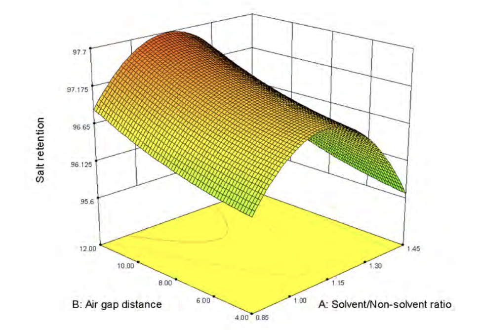
The retention and flux, obtained from earlier experiments, support the findings from the analysis of variance, which shows that solvent/non-solvent and bore fluid ratio are important factors that affect the membrane performance. The retention and flux plots show an improvement in salt retention and water flux as the solvent/non-solvent ratio in the solution was decreased from 1.447 to 1.147 (factor A) while decreasing the solvent concentration (factor c) in the bore fluid. The decrease in solvent/non-solvent ratio will result in a high formamide ratio in the spinning solution, which will shift the composition path of the spinning solution in the direction of the liquid-liquid demixing gap and as a result, a porous membrane will be produced. The decrease of acetone in the bore fluid from 70 to 60 and 50% (m/m) will improve the flux and retention of the produced hollow-fine fibres. High solvent concentration in the bore fluid and dope solution produced a very thick dense layer when the extruded fibres undergo rapid phase separation from both sides. The formation of an impermeable skin is due to the high gelation of supersaturated top layer of the spinning solution. Lowering the solvent concentration by increasing the non-solvent content in both bore fluid and the spinning solution will slow down and control the two different processes of gelation and the phase separation process and hence, more porous hollow-fine fibres could be produced with improved flux and retention. Figures 5 and 6 illustrate the interaction plot between solvent/non-solvent ratio and air gap distance on both retention and flux.
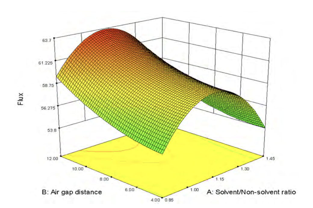
It is clear that both flux and retention were increased with decreasing the solvent/non- solvent ratio and increasing the air gap distance to 120 mm. It was stated that the air gap is responsible for the formation of a thin skin on the outside of the fibre and the bulk of membrane structure is formed in the coagulation bath. Then increasing the non-solvent content in the spinning solution with 12 cm air gap distance will produce very thin skin layer with more pores in it. As the composition bath of the spinning solution will become close to the liquid-liquid demixing state with high non-solvent content, the spinodal outer layer should result in a microporous skin layer. Fibres spun with different air gap distances experience elongational stress with higher take-up speeds that induce molecular orientation and cause polymer molecules to pack more closely to one another. For a small air gap distance 4 cm, there was too little time for orientation and with a high take-up speed leading to a much tighter structure resulted. With an air gap of 12 cm the orientation will have small relaxation time before entering the gelation bath, leading to a less dense outer skin and subsequently high flux and retention. Figure 7 and 8 illustrate the interaction plot between the air gap distances and bore fluid ratio on both retention and flux.
It can be seen the bore fluid ratio had a large effect on flux. This can be explained that higher air gap distance results in enough time for the mass transfer at the inner surface, which means enough time for bore liquid/solvent exchange. As a result, an open porous structure will be formed on the inner surface leading to an increase in the flux.
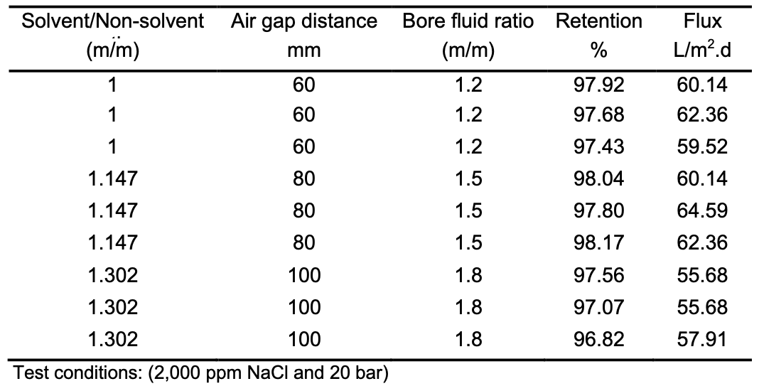
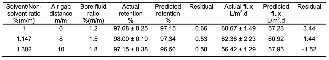
Model validation In order to verify the adequacy of the model developed, three confirmation experiments were conducted within the range of the levels studied. Each of the experiments was repeated three times from different dope solutions and the average was taken for the retention and flux of each experiment. For each of the confirmations, the responses were determined experimentally and calculated by using the regression equation. The results of these validation experiments and the model predicted values are shown in Table 6.
The average values are shown in Table 7 for each set together with their predicted values calculated from the regression model. The results showed that our regression model yields reasonable results for the flux and retention with small residual between predicted and actual data. Therefore, our regression equation can be expected to apply in the preparation of CA hollow-fine-fibre membranes with better performance.
Conclusions In this study, the ability of a factorial design to perform a comparative investigation of the importance of individual factors and their interactions on the membrane performance was demonstrated. It was concluded in this statistical analysis that the solvent/non-solvent ratio, bore fluid ratio, air gap distance and the interaction between solvent/non-solvent and bore fluid, air gap distance, and bore fluid ratio had a significant influence on both the flux and retention of CA hollow-fine-fibre membranes for brackish water desalination. According to 33 factorial designs, the regression analysis showed a goodness of fit to the experimental data. Therefore, the model was considered adequate for the prediction of good membrane performance (salt retention in the range of 96 – 98% and permeate flux in the range of 60 – 64 L/m2.d.
References
|
|||||||||||||||||||||||||||||||||||||||||||||||||